Direct problem: modeling pheromone propagation

import numpy as np
import matplotlib.pyplot as plt
import matplotlib.ticker as ticker
from pathlib import Path
import os
import time

import pherosensor

from pheromone_dispersion.geom import MeshRect2D
from pheromone_dispersion.diffusion_tensor import DiffusionTensor
from pheromone_dispersion.velocity import Velocity
from pheromone_dispersion.source_term import Source
from pheromone_dispersion.convection_diffusion_2D import DiffusionConvectionReaction2DEquation

from utils.plot_env_param import plot_velocity_field, plot_diffusion_tensor
from utils.plot_colormap import plot_colormap, plot_colormap_all_timestep
from utils.generate_gif import generate_gif

path = os.getcwd()
path_data = path + '/data'
path_output = path + '/output'
if not os.path.isdir(Path(path_output)):
    os.makedirs(Path(path_output))
path_plot = path_output + '/plot'
if not os.path.isdir(Path(path_plot)):
    os.makedirs(Path(path_plot))

This notebook aims at presenting the Partial Differential Equations (PDE) used to model the pheromone propagation in the atmosphere, the solvers implemented in the module pheromone_dispersion and the different submodules on which the solvers are based.

In a first section, the 2D PDE pheromone propagation model is presented.

Then, the different submodules are presented and illustrated over a simple but representative case.

At last but not at least, the numerical solvers of the PDE model are presented and used to model the pheromone propagation in this test case.

bibliography: ../paper/paper.bib

Pheromone propagation model

The most classical model to simulate propagation of chemical specie in the atmosphere is a 3D Chemical-Transport Model (CTM). The CTM are obtained from the reactive Navier-Stokes equations by using especially the dilution hypothesis. This hypothesis consists in decoupling the dynamic of the atmosphere and the dynamic of the concentration of the chemical specie that is present is very small proportion and assumed chemically passive. As consequence, dynamical field such as the wind or the diffusion coefficients can be computed separately and given as parameters of the CTM.

In the present context, the following 2D depth-integrated CTM, referred as the pheromone propagation model below, is used to model the total concentration of pheromone over the depth of the layer \(c(x,y,t)\) [\(g.m^{-2}\)] on a domain \(\Omega\in\mathbb{R}^2\) and during a time window \([0;T]\).

\[\begin{equation} \frac{\partial c}{\partial t}-\nabla\cdot(\mathbf{K}\nabla c)+\nabla\cdot(\vec{u}c)+\tau_{loss}c=s~\forall (x,y,t)\in\Omega\times[0;T] \end{equation}\]

The coefficient \(\mathbf{K}(x,y,t)\) [\(m^2.s^{-1}\)] is the diffusion coefficient. This coefficient results from modelling the turbulent diffusion at an unresolved scale (classically, scale smaller than the scale of the numerical grid) using the K theory.

As mentioned above, in CTM, the wind velocity field \(\vec{u}(x,y,t)=(u(x,y,t),v(x,y,t))\) [\(m.s^{-1}\)] is given as parameter. For example, \(\vec{u}\) can be computed using a large meteorological model and then, taken as input data in the present CTM.

The loss coefficient \(\tau_{loss}(x,y,t)\) [\(s^{-1}\)] is the coefficient resulting from the loss of pheromone due to vertical phenomena. This includes the deposition and settling of the pheromone on the ground and the vertical diffusion that will spread the pheromone out of the layer of interest. Let us note that the loss coefficient \(\tau_{loss}\) depends on the vegetation presents on the ground and on the stability of the atmosphere.

The source term \(s(x,y,t)\) [\(g.m^{-2}.s^{-1}\)] of the pheromone propagation model is the quantity of pheromone emitted by the insects per second. In the context of the PheroSensor project, the source term \(s\) is the quantity to infer to deduce the localization of the insects. This inference is the subject of the package source_localization presented in the notebook on pheromone emission inference and source localization.

The pheromone propagation model is closed by the following initial and boundary conditions:

• a null initial condition \(c(x,y,t=0)=0~\forall (x,y)\in\Omega\),

• a null diffusive flux \(\mathbf{K}\nabla c\cdot\vec{n}=0\) \(\forall (x,y)\in\partial\Omega\),

• a null entering convective flux \(\vec{u}c\cdot\vec{n}=0\) \(\forall (x,y)\in\partial\Omega\cap \{(x,y)|\vec{u}(x,y,t)\cdot\vec{n}<0\}~\forall t\in]0;T]\) with \(\vec{n}\) the outgoing normal vector.

The pheromone propagation model is solved using implicit and semi-implicit upwind finite volume schemes implemented. More details can be found in the notebooks located in the folder ./test_numerical_scheme/ that introduce and test the numerial scheme, including convergence, and the solvers.

More details on this model and its derivation can be found in Malou et al (2024).

Construction of the solver of the pheromone propagation model

Specifying the geometry using the geom submodule

For now, the numerical solver of the pheromone propagation model has been implemented for a rectangular domain \(\Omega=[0;L_x]\times[0;L_y]\). Moreover, the mesh is supposed to be cartesian (rectangular cells) with constant space steps \(\Delta x\) and \(\Delta y\).

Such geometry can be generated as an object of the MeshRect2D class of the geom submodule.

Lx = 30 # the length along the x-axis
Ly = 40 # the length along the y-axis
Delta_x = 0.5 # the space step along the x-axis
Delta_y = 0.5 # the space step along the y-axis
T_final = 20 # the final time of the simulation
msh = MeshRect2D(Lx, Ly, Delta_x, Delta_y, T_final)

Once the geometry is initialized, it remains to compute time step \(\Delta t\) and the resulting array containing the time point. The time step is chosen especially to satisfy numerical stability conditions depending on the chosen time discretization (see below).

In case of a implicit time discretization, the time step should be given by the user as the numerical scheme is unconditionnally stable. To do so, the user can use the calc_dt_implicit_solver method of the MeshRect2D class.

In case of a semi-implicite or explicite time discretization, the user can use the calc_dt_explicit_solver method of the MeshRect2D class to compute a time step that satisfies the CFL condition depending on the wind field (see below).

msh.calc_dt_implicit_solver(.1)

Specifying the wind velocity field using the velocity submodule

As mentionned previously, the wind velocity field \(\vec{u}=(u,v)\) has to be given as parameter of the pheromone propagation model.

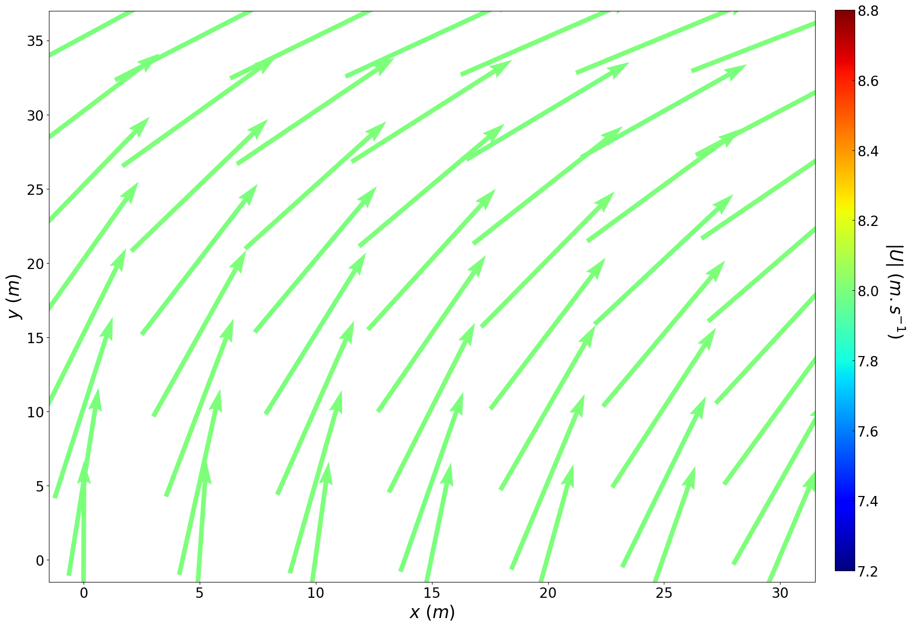
The wind field is here contained in an object of the Velocity class of the velocity submodule. As the solvers are based on the finite volume method (see more details in this notebook), the velocity field should be given at both the vertical and horizontal interfaces of the cells of the mesh. One can provide stationnary wind field. Otherwise, the time array should be specified and between two time points contained in this array, the wind field will be linearly interpolated.

Thus, the user should provide arrays containing the wind field at the vertical interface and at the horizontal interface that are resp. of shape (nb cell in y axis, nb cell in x axis + 1, 2) and (nb cell in y axis + 1, nb cell in x axis, 2) if the wind field is stationnary, and of shape (nb time point, nb cell in y axis, nb cell in x axis + 1, 2) and (nb time point, nb cell in y axis + 1, nb cell in x axis, 2) otherwise.

U_vi = np.load(Path(path_data) / f'U_vi.npy')
U_hi = np.load(Path(path_data) / f'U_hi.npy')
U = Velocity(msh,U_vi, U_hi)

The Velocity class also contains useful attributes and methods to manipulate the wind field. For instance, the attributes at_vertical_interface and at_horizontal_interface contain the velocity field at resp. the vertical and horizontal interfaces of the mesh’s cells at the current time, and the method at_current_time enables to update all the attributes at the time given as input of the method.

Moreover, the wind velocity field can be plotted at the current time using the plot_velocity_field method of the utils module.

plot_velocity_field(msh,U)

The velocity submodule also containes a velocity_field_from_meteo_data method that can be used to generate an object of the Velocity class from meteorological data contained in a .csv file whose path and name are given as input.

This method is implemented for meteorological data in the format of the data provided by the AROME model of MeteoFrance. However, it can easily be adapted for other format.

This method computes the wind field on each cell interfaces by linear interpolation of the data potentially located on a irregular grid.

Specifying the diffusion tensor using the diffusion_tensor submodule

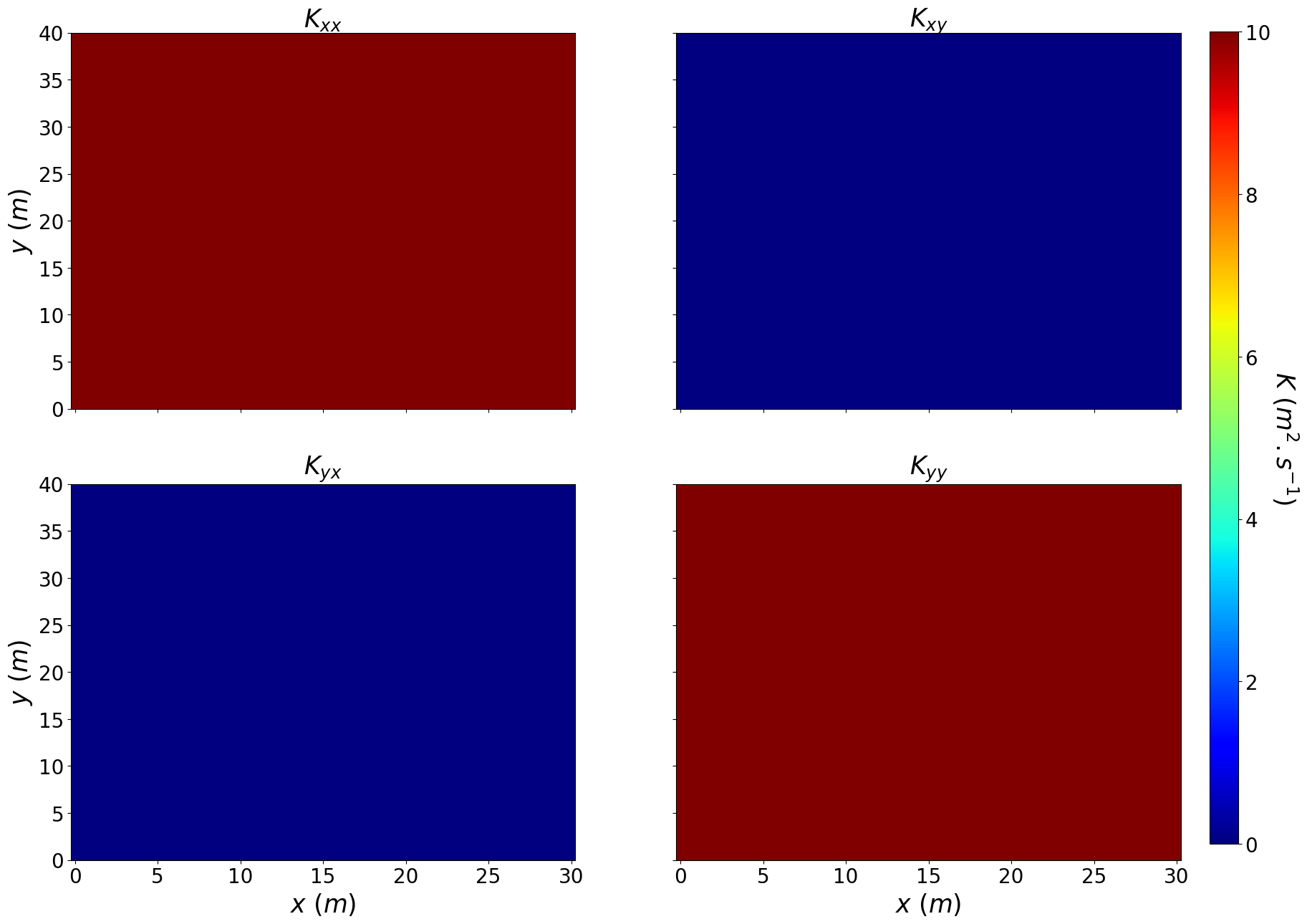
The diffusion tensor is here contained in an object of the DiffusionTensor class of the diffusion_tensor submodule.

In the present case, we suppose that the diffusion tensor is given by a diffusion coefficient \(K_u\) in the wind direction and a diffusion coefficient \(K_{u^\perp}\) in the crosswind direction.

Hence, the anistropic diffusion tensor is given by \(\mathbf{K} = R(U)diag(K_u,K_{u^\perp})R(U)^T\) with \(R(U)\) the rotation matrice of angle \(\theta\) between the wind field and the cartesian frame. By the definition of the rotation matrice, the diffusion tensor can be rewritten \(\mathbf{K} = K_{u^\perp}Id + (K_u-K_{u^\perp})\frac{UU^T}{\|U\|^2}\).

Let us note that, in general, the crosswind diffusion coefficient \(K_{u^\perp}\) is much larger that the wind diffusion coefficient.

Thus, the user should provide an object of the class velocity and the “in the wind direction” and the cross-wind diffusion coefficients to instanciate an object of the class diffusion_tensor.

For now, the case of a non-diagonal \(\mathbf{K}\) has not been implemented. Therefore, we will take \(K_u=K_{u^\perp}\).

K = DiffusionTensor(U, 10., 10.)

As the numerical scheme is a finite volume scheme (see more details in this notebook) and similarly to the class Velocity, the DiffusionTensor class contains the attributes at_vertical_interface and at_horizontal_interface contain the diffusion tensor at resp. the vertical and horizontal interfaces of the mesh’s cells at the current time, and the method at_current_time enables to update all the attributes at the time given as input of the method.

Moreover, the user can plot the diffusion tensor maps at the current time using the plot_diffusion_tensor method of the module utils

plot_diffusion_tensor(msh, K)

Specifying the loss coefficient

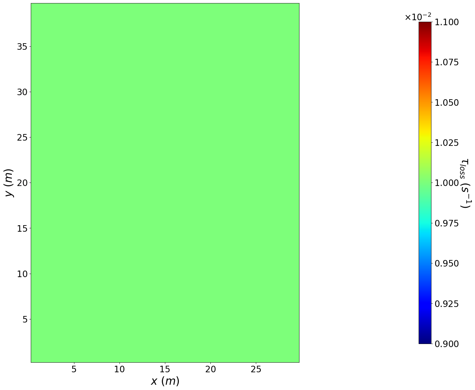
The loss coefficient is here simply contained in a array of shape (nb cell in y axis, nb cell in x axis) that is the average loss coefficient over a cell and that the user should provide.

loss_coeff = 0.01*np.ones((msh.y.size, msh.x.size))

Moreover, the user can plot the loss coefficient map using the plot_colormap method of the module utils.

plot_colormap(msh,loss_coeff,'\\tau_{loss}', 's^{-1}', cmap="jet")#, save_path=path_plot

As mentionned earlier, the loss coefficient depends on the vegetation covering the ground. With this in mind, the submodule deposition_coefficient contains the method deposition_coeff_from_land_occupation_data that return the loss coefficient map given a file containing land occupation data and a dictionnary containing the loss coefficient depending on the land occupation.

Let us note that the keyword of the columns containing the polygon and the land occupation classification of the land occupation data may vary depending on the format. However, the method can be easily modified to match a given format.

Specifying the pheromone emission using the source_term submodule

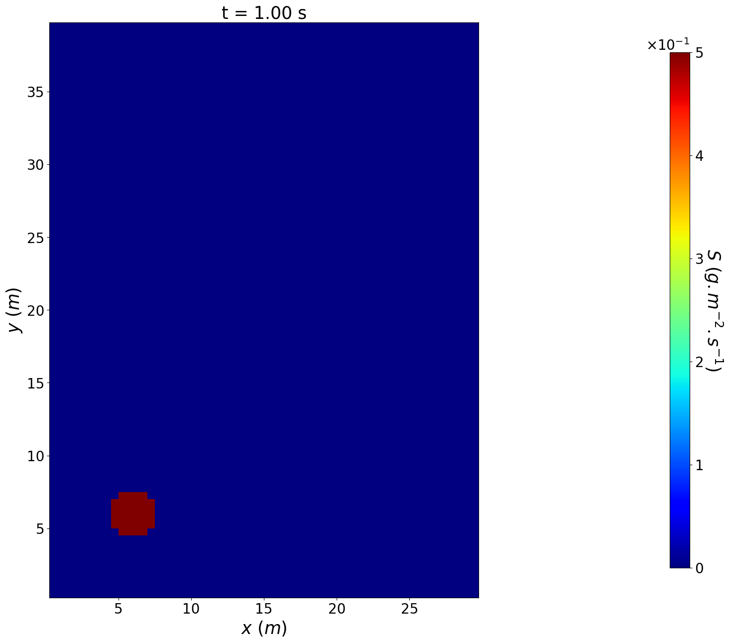
The last element of the pheromone propagation model is the source term that is the quantity of pheromone emitted by the pest insect that should be provided by the user when modelling the propagation of pheromone in the atmosphere. The source term is contained in an object of the Source class contained in the source_term submodule.

As for the wind field, one can provide stationnary source term and otherwise, the time array should be specified and between two time points contained in this array, the source term will be linearly interpolated.

Thus, the user should provide an array containing the source term at each cells of the mesh that is of shape (nb cell in y axis, nb cell in x axis) if the source term is stationnary, and of shape (nb time point, nb cell in y axis, nb cell in x axis) otherwise.

amp = 0.5
xc = 6.
yc = 6.
r = 1.5# 2 #
S_value = np.zeros((msh.t_array[::2].size, msh.y.size, msh.x.size))
xx, yy= np.meshgrid(msh.x, msh.y)
S_value[:, (xx-xc)**2 + (yy-yc)**2 < r**2] = amp

S = Source(msh, S_value, t=msh.t_array[::2])

Moreover, the user can plot the source term at a given time using the plot_colormap method of the module utils.

t_on = 1.
S.at_current_time(t_on)
plot_colormap(msh,S.value,'S', 'g.m^{-2}.s^{-1}', cmap="jet",title=f't = {"{:.2f}".format(t_on)} s')

As for the class Velocity and the class DiffusionTensor, the class Source contains the method at_current_time that enables to update all the attributes at the time given as input of the method.

Specifying the pheromone propagation model and its solver using the convection_diffusion_2D submodule

The pheromone propagation model is contained in an object of the class DiffusionConvectionReaction2DEquation of the convection_diffusion_2D submodule.

In addition to the wind field, diffusion tensor, loss coefficient and source term that have been specified above, the user can specify the type of time discretization (see more details below and in this notebook on the numerical scheme) and the relative tolerance of the resolution of the linear system at each time step.

solver = 'implicit with stationnary matrix inversion'
tol = 1e-10
EDP = DiffusionConvectionReaction2DEquation(
    U,
    K,
    loss_coeff,
    S,
    msh,
    tol_inversion=tol,
    time_discretization=solver
)

Multiple solver types have been implemented in the class DiffusionConvectionReaction2DEquation and the associated keyword can be found in the attribute implemented_solver_type.

print(EDP.implemented_solver_type)

['implicit', 'semi-implicit', 'semi-implicit with matrix inversion', 'implicit with stationnary matrix inversion']

With the implicit and semi-implicit time discretization, the resolution of the linear system at each time step are based on resp. a GMRES algorithm and a conjugate gradient algorithm.

With the time discretization with matrix inversion, the matrices of the linear system to solve are inverted once and for all and then, the resolution of the linear system at each time step is reduced to a matrix-vector product.

In this case, the user should use the method init_inverse_matrix of the class DiffusionConvectionReaction2DEquation. With this method, the user specifies the path and name of the file containing the inverse matrix. If the inverse matrices have already been computed and stored in the specified file, then the method load the matrices. If the inverse matrices are not found in the folder, then the method computes and store them once and for all.

This is particularly efficient when the wind is assumed stationnary and so the matrix to invert is the same at each time step. This case is implemented under the keyword implicit with stationnary matrix inversion and is used in this test case.

fname = 'inv_matrix_implicit_solver'
EDP.init_inverse_matrix(path_to_matrix=path_data, matrix_file_name=fname)

=== Computation of the inverse of the matrix of the implicit part of the implicit with stationnary matrix inversion scheme ===
--- Computation at time t=  0 in  11.089861392974854  s

Solving the PDE to model the pheromone propagation and plot the pheromone concentration

The pheromone propagation can be solved using the solver method.

This method aims at computing the pheromone concentration on the whole domain and at time steps given a store rate, for instance a store rate of 10 will imply one time out of ten will be returned and saved. The user can use optional inputs to save the results in a given folder.

if not (Path(path_output) / 'c_save.npy').exists():
    t_0 = time.time()
    store_rate = 10
    t_output, c_output = EDP.solver(save_flag=True, path_save=path_output, store_rate=store_rate)
    t_f = time.time()
    print("")
    print("--- resolution of the direct model in %s seconds ---" % (t_f - t_0) )
else:
    print("--- the resolution has already been performed ---")
    c_output = np.load(Path(path_output) / f'c_save.npy')
    t_output = np.load(Path(path_output) / f't_save.npy')

t = 20.000 / 20.000 s
--- resolution of the direct model in 3.335312843322754 seconds ---

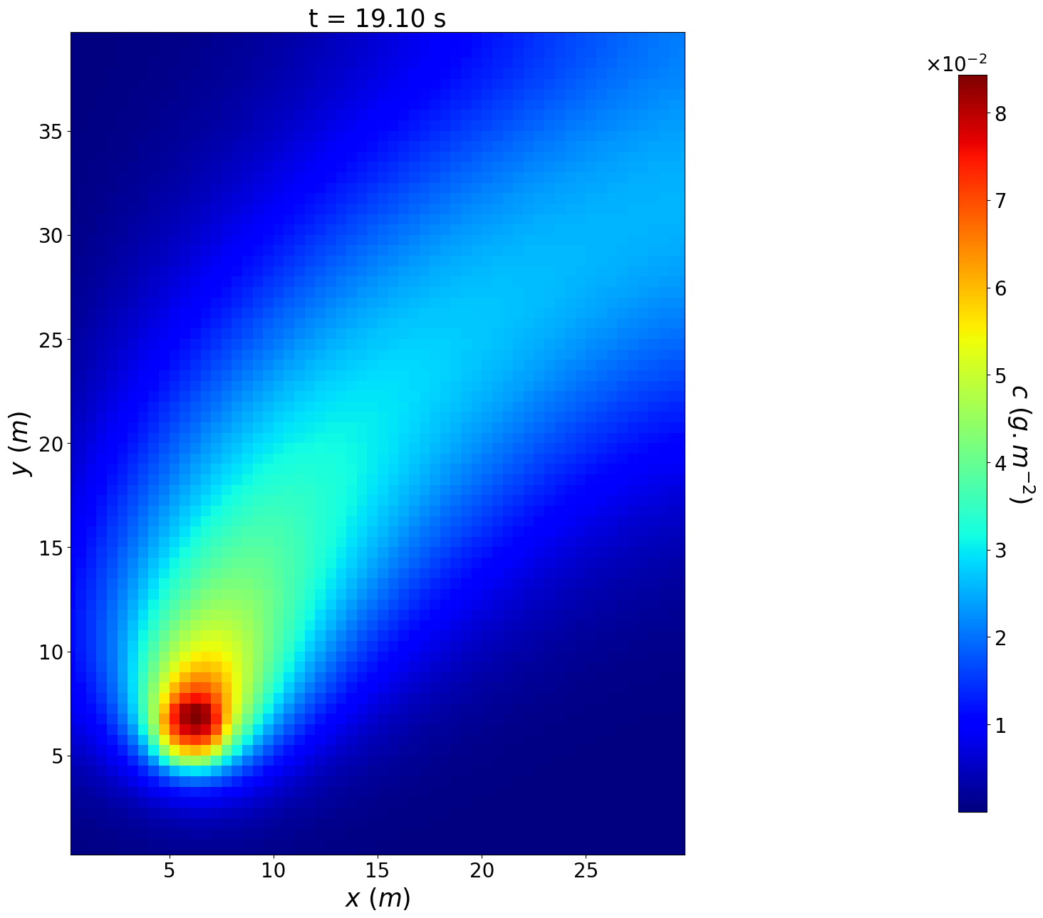
The resulting pheromone concentration map can easily be plotted at a given time using the plot_colormap method of the module utils.

t_plot = 20.
i = np.argmin(np.abs(t_output-t_plot))
plot_colormap(msh,c_output[i,:,:],'c', 'g.m^{-2}', cmap="jet",title=f't = {"{:.2f}".format(t_output[i])} s')#, save_path=path_plot

n_col = 5
n_ligne = t_output.size//n_col

fontsize=25
xv, yv = np.meshgrid(msh.x, msh.y, sparse=True, indexing="ij")
vmin = np.min(c_output)
vmax = np.max(c_output)
fig, axs = plt.subplots(n_ligne,n_col,figsize=(20,15), sharex=True, sharey=True)

for i, t in enumerate(t_output):

    l = i//n_col
    c = i%n_col
    title = f'at t = {"{:.1f}".format(t)} s'
    fmt = ticker.LogFormatterMathtext()
    fmt.create_dummy_axis()
    levels = [10**(i) for i in [-4,-3,-2,-1,0]]
    c_plot = c_output[i,:,:]
    contour = axs[l,c].contour(msh.x-np.min(msh.x), msh.y-np.min(msh.y), c_plot, linestyles='dashed', levels=levels, linewidths=2)
    axs[l,c].clabel(contour, inline=True, fontsize=10, fmt=fmt)
    pcmesh = axs[l,c].pcolormesh(xv[:, 0]-np.min(msh.x), yv[0, :]-np.min(msh.y), c_plot, cmap='jet', vmin=vmin, vmax=vmax)
    axs[l,c].set_aspect('equal', adjustable='box')
    axs[l,c].set_title(title, fontsize=fontsize - 5)
    axs[l,c].set_xticks([0,20,40])
    axs[l,c].set_yticks([0,20,40,60])
    axs[l,c].tick_params(labelsize=fontsize - 5)
    axs[l,c].set_xlim(0.,np.max(msh.x)-np.min(msh.x))
    axs[l,c].set_ylim(0.,np.max(msh.y)-np.min(msh.y))

fig.supxlabel('$x$ ($m$)', fontsize=fontsize)
fig.supylabel('$y$ ($m$)', fontsize=fontsize, x=0.08, y=0.5)
cbar_ax = fig.add_axes([0.91, 0.117, 0.015, 0.755])
cbar = fig.colorbar(pcmesh, cax=cbar_ax)
cbar_ax.tick_params(labelsize=fontsize - 5)
cbar.set_label('$c$ ($pg.m^{-2}$)', rotation=270, fontsize=fontsize, labelpad=40)
plt.show()

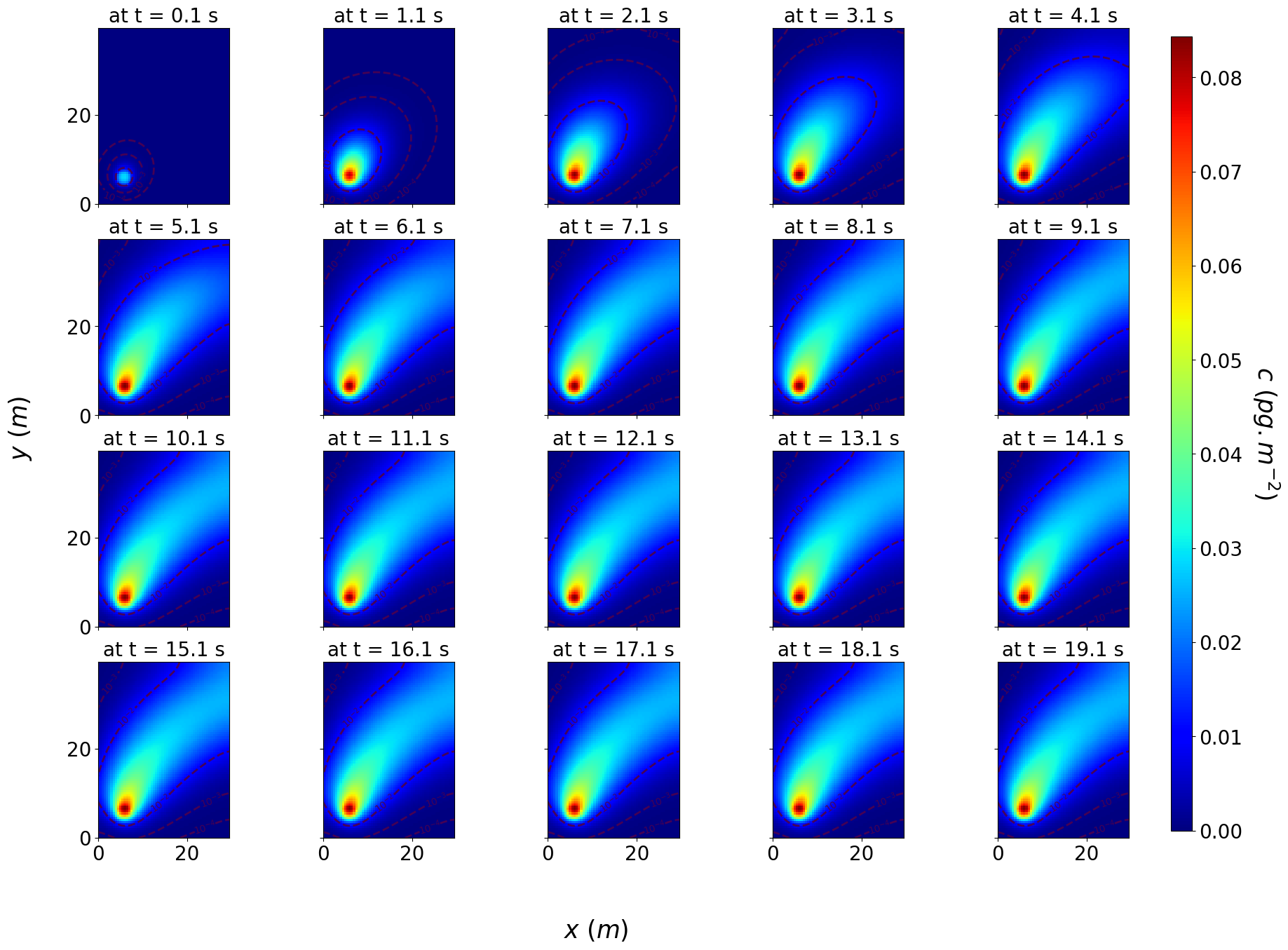
One can also plot multiple time step using the plot_colormap_all_timestep method and generate a gif using these plots and the method generate_gif of the module utils.

path_plot_all_timestep = path_plot + '/plot_all_timestep'
if not os.path.isdir(Path(path_plot_all_timestep)):
    os.makedirs(Path(path_plot_all_timestep))
plot_colormap_all_timestep(msh,t_output,c_output,'c', 'g.m^{-2}', cmap="jet", save_path=path_plot_all_timestep)

 ite = 20 / 20

generate_gif(images_path=path_plot_all_timestep, save_path=path_plot, file_name='output_pheromone_propagation')

 100% : saving the gifg