[1]:
import matplotlib.pyplot as plt
from matplotlib import ticker
import numpy as np
import numpy.linalg as npl

import pherosensor

from pheromone_dispersion.advection_operator import Advection
from pheromone_dispersion.geom import MeshRect2D
from pheromone_dispersion.velocity import Velocity
[2]:
Lx = 20
Ly = 25
Delta_x = 0.4
Delta_y = 0.4
T_final = 5.
Test of the numerical scheme of the advection operator
This notebook aims to test the implementation of the numerical scheme of the advection operator.
The advection operator is the operator \(A:c(x,y)\mapsto \nabla\cdot(U(x,y) c(x,y))~\forall (x,y)\in\Omega\) such that \(U(x,y)c(x,y)\cdot \vec{n} = 0~\forall(x,y)\in\partial\Omega_i\) with \(\partial\Omega_i = \{ (x,y)\in\partial\Omega, U(x,y)\cdot\vec{n}<0\}\).
Reference solution
We consider the reference solution \(c^{ref}(x,y) = sin\left(\frac{2\pi n_x}{L_x}x\right)sin\left(\frac{2\pi n_y}{L_y}y\right)\)
[3]:
nx = 5
ny = 7
lambda_x = 2 * np.pi * nx / Lx
lambda_y = 2 * np.pi * ny / Ly

def c_reference(x,y):
    return np.sin(lambda_x * x) * np.sin(lambda_y * y)
and the velocity \(U(x,y)=(u,v)(x,y)=(\frac{3}{L_x}x, \frac{4}{L_y}y)\).
[4]:
def u(x):
    return 3*x/Lx

def v(y):
    return 4*y/Ly

def velocity_field(msh):
    x, yi = np.meshgrid(msh.x, msh.y_horizontal_interface)
    U_hi = np.zeros((msh.y_horizontal_interface.size,msh.x.size,2))
    U_hi[:,:,0] = u(x)
    U_hi[:,:,1] = v(yi)

    xi, y = np.meshgrid(msh.x_vertical_interface, msh.y)
    U_vi = np.zeros((msh.y.size,msh.x_vertical_interface.size,2))
    U_vi[:,:,0] = u(xi)
    U_vi[:,:,1] = v(y)

    return Velocity(msh, U_vi, U_hi)
Hence, we have \(Ac^{ref}(x,y) = \nabla\cdot(U c^{ref})(x,y) = \frac{3}{L_x}\left(\frac{2\pi n_x}{L_x}xcos\left(\frac{2\pi n_x}{L_x}x\right)+sin\left(\frac{2\pi n_x}{L_x}x\right)\right)sin\left(\frac{2\pi n_y}{L_y}y\right) + \frac{4}{L_y}\left(\frac{2\pi n_y}{L_y}ycos\left(\frac{2\pi n_y}{L_y}y\right)+sin\left(\frac{2\pi n_y}{L_y}y\right)\right)sin\left(\frac{2\pi n_x}{L_x}x\right)\)
[5]:
def Ac_reference(x,y):
    res = (3 / Lx) * ( lambda_x * x * np.cos(lambda_x * x) + np.sin(lambda_x * x) ) * np.sin(lambda_y * y)
    res+= (4 / Ly) * ( lambda_y * y * np.cos(lambda_y * y) + np.sin(lambda_y * y) ) * np.sin(lambda_x * x)
    return res
Numerical scheme
if \(U_{i\pm1/2,j}\cdot \vec{n} = u_{i\pm1/2,j} > 0\), then \(c_{i\pm1/2,j} = c_{i\pm1/2-1/2,j}\), else \(c_{i\pm1/2,j} = c_{i\pm1/2+1/2,j}\),
if \(U_{i,j\pm1/2}\cdot \vec{n} = v_{i,j\pm1/2} > 0\), then \(c_{i,j\pm1/2} = c_{i,j\pm1/2-1/2}\), else \(c_{i,j\pm1/2} = c_{i,j\pm1/2+1/2}\).
[6]:
space_factor_a = [0.005, 0.01, 0.1, 1.]
dx_a = np.zeros(len(space_factor_a))

MAE = np.zeros(len(space_factor_a))
RMSE = np.zeros(len(space_factor_a))

for i, space_factor in enumerate(space_factor_a):

    msh = MeshRect2D(Lx, Ly, Delta_x*space_factor, Delta_y*space_factor, T_final)
    x, y = np.meshgrid(msh.x, msh.y)
    dx_a[i] = Delta_x*space_factor

    c_ref = c_reference(x, y)
    Ac_ref = Ac_reference(x,y)

    U = velocity_field(msh)
    A = Advection(U, msh)
    Ac_solver = A.matvec(c_ref.reshape((msh.y.size * msh.x.size,)))
    Ac_solver = Ac_solver.reshape((msh.y.size, msh.x.size))

    RMSE[i] = npl.norm(Ac_solver - Ac_ref) / np.sqrt(Ac_ref.size)
    MAE[i] = np.mean(np.abs(Ac_solver-Ac_ref))

    print("")
    print("dx = ", msh.dx)
dx =  0.002

dx =  0.004

dx =  0.04000000000000001

dx =  0.4
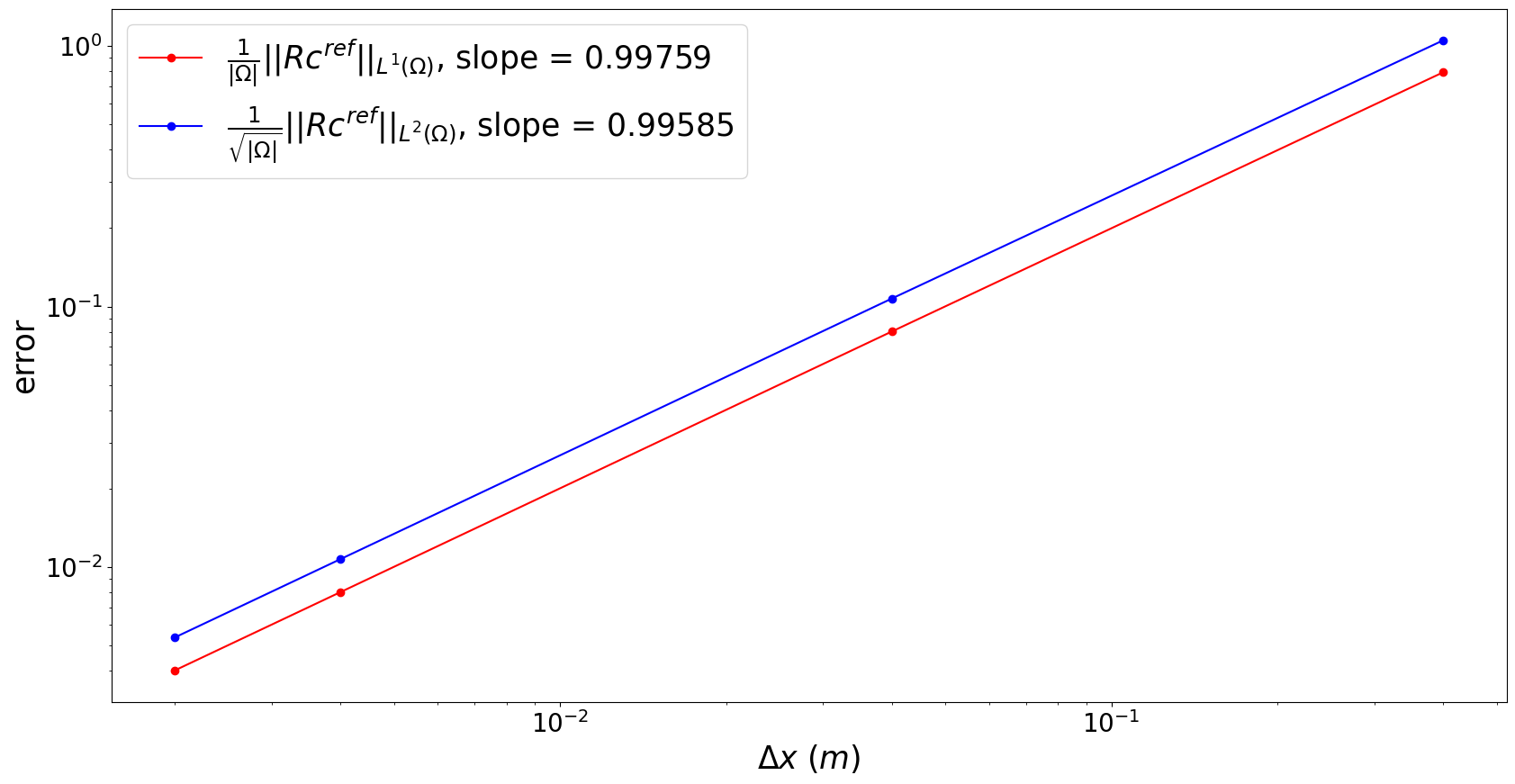
Analysis of the truncation error
[7]:
slope_MAE = (np.log(MAE[0]) - np.log(MAE[-1])) / (np.log(dx_a[0]) - np.log(dx_a[-1]))
slope_RMSE = (np.log(RMSE[0]) - np.log(RMSE[-1]) ) / ( np.log(dx_a[0]) - np.log(dx_a[-1]))

fontsize = 25
fig, ax1 = plt.subplots(figsize=(20, 10))
ax1.plot(dx_a,MAE,'-or',label=r'$\frac{1}{|\Omega|}||Rc^{ref}||_{L^1(\Omega)}$'+f', slope = {"{:.5f}".format(slope_MAE)}')
ax1.plot(dx_a,RMSE,'-ob',label=r'$\frac{1}{\sqrt{|\Omega|}}||Rc^{ref}||_{L^2(\Omega)}$'+f', slope = {"{:.5f}".format(slope_RMSE)}')
ax1.tick_params(axis='both',labelsize=fontsize-5)
ax1.set_ylabel(r'error', fontsize=fontsize)
ax1.set_xlabel('$\Delta x$ ($m$)', fontsize=fontsize)
ax1.set_xscale('log')
ax1.set_yscale('log')
ax1.legend(loc='upper left',prop={'size': fontsize})
[7]:
<matplotlib.legend.Legend at 0x79247ba168d0>