[1]:

import matplotlib.pyplot as plt
import numpy as np
import numpy.linalg as npl
from scipy.sparse.linalg import cg

import pherosensor

from pheromone_dispersion.convection_diffusion_2D import DiffusionConvectionReaction2DEquation, Source
from pheromone_dispersion.diffusion_tensor import DiffusionTensor
from pheromone_dispersion.geom import MeshRect2D
from pheromone_dispersion.velocity import Velocity

from source_localization.cost import Cost
from source_localization.control import Control
from source_localization.adjoint_convection_diffusion_2D import AdjointDiffusionConvectionReaction2DEquation
from source_localization.obs import Obs

[2]:

Lx = 20#50 # the length along the x-axis
Ly = 25#60 # the length along the y-axis
Delta_x = 1. # 0.4 the space step along the x-axis
Delta_y = 1. # 0.4 the space step along the y-axis
T_final = 2. # the final time of the simulation

Test of the numerical scheme of the adjoint model

This notebook aims to test the numerical scheme of the direct model and its implementation by comparing the results of the numerical solver with a reference solution used to derive an associated source term.

Reference solution

In the present case, we consider a velocity field of shape \(U(x,y) = (u(x,y),0)^T\) (with \(u\geq0\)) with the horizontal velocity \(u(x,y)=\frac{4}{L_x^2}(x-L_x)^2\frac{3}{2L_y}y\). Let us note that this velocity satisfies \(u\geq0\) and \(up = 0\) at \(x=L_x\).

[3]:

def velocity_horizontal(x,y):
    xx, yy = np.meshgrid(x, y)
    return 4 * (xx - Lx)**2 * 3 * yy / (Lx**2 * 2 * Ly)

def velocity_field(msh):

    U_hi = np.zeros((msh.y_horizontal_interface.size, msh.x.size,2))
    U_hi[:,:,0] = velocity_horizontal(msh.x, msh.y_horizontal_interface)

    U_vi = np.zeros((msh.y.size, msh.x_vertical_interface.size,2))
    U_vi[:,:,0] = velocity_horizontal(msh.x_vertical_interface, msh.y)

    return Velocity(msh, U_vi, U_hi)

The diffusion tensor is considered of shape \(K=diag(K_x,K_y)\) with constant \(K_x\) and \(K_y\) and the reaction coefficient constant.

[4]:

K_x = 5./6  # diffusion coefficient in the crosswind direction (less weak)
K_y = 0.01  # diffusion coefficient in the downwind direction (very weak)
tau_loss = 10

Hence, the 2D PDE reduces to \(\partial_tp+u\partial_xp+K_x\partial_{xx}p+K_y\partial_{yy}p-\tau_{loss}p = \big(\partial_cd(c(s))\big)^*\cdot\nabla_dJ\big(s,d(c(s))\big)\)
with the final condition: \(p(t=T)=0\),
the boundary conditions:
\(K_x\partial_xp = 0\) at \(x = 0\) and \(x = L_x\),
\(K_y\partial_yp = 0\) at \(y = 0\) and \(y = L_y\),
and \(up = 0\) at \(x= 0\).

We consider the reference solution \(p^{ref}(x,y,t) = (T-t)\left(cos\left(\frac{2\pi n_xx}{L_x}\right)+cos\left(\frac{2\pi n_yy}{L_y}\right)\right)\) with \(n_x\) and \(n_y\) two integers.

Let us note that the boundary conditions \(K_x\partial_xc = 0\) at \(x = 0\) and \(x = L_x\), \(K_y\partial_yc = 0\) at \(y = 0\) and \(y = L_y\) are then satisfied.

[5]:

nx = 1
ny = 3
lambda_x = 2 * np.pi * nx / Lx
lambda_y = 2 * np.pi * ny / Ly

def p_reference(msh):
    xx, yy = np.meshgrid(msh.x, msh.y)
    p_ref = np.zeros((msh.t_array.size, msh.y.size, msh.x.size))

    for it,t in enumerate(msh.t_array):
        p_ref[it,:,:] = (msh.T_final - t) * ( np.cos(lambda_x * xx) + np.cos(lambda_y * yy) )

    return p_ref

From this reference solution, we have :
\(\partial_tp^{ref}(x,y,t) = - cos\left(\frac{2\pi n_xx}{L_x}\right) - cos\left(\frac{2\pi n_yy}{L_y}\right)\)
\(\partial_xp^{ref}(x,y,t)=-(T-t)\frac{2\pi n_x}{L_x}sin\left(\frac{2\pi n_xx}{L_x}\right)\), \(\partial_{xx}p^{ref}(x,y,t)=-(T-t)\frac{4\pi^2 n_x^2}{L_x^2}cos\left(\frac{2\pi n_xx}{L_x}\right)\)
\(\partial_yp^{ref}(x,y,t)=-(T-t)\frac{2\pi n_y}{L_y}sin\left(\frac{2\pi n_yy}{L_y}\right)\), \(\partial_{yy}p^{ref}(x,y,t)=-(T-t)\frac{4\pi^2 n_y^2}{L_y^2}cos\left(\frac{2\pi n_yy}{L_y}\right)\)
Hence, we have the associated source term: \begin{align*}
\Sigma=\big(\partial_cd(c(s))\big)^*\cdot\nabla_dJ\big(s,d(c(s))\big) (x,y,t) = &-\left(1+\tau_{loss}(x,y)(T-t)+K_x(T-t)\frac{4\pi^2 n_x^2}{L_x^2}\right)cos\left(\frac{2\pi n_xx}{L_x}\right)\\
          &- \left(1+\tau_{loss}(x,y)(T-t)+K_y(T-t)\frac{4\pi^2 n_y^2}{L_y^2}\right)cos\left(\frac{2\pi n_yy}{L_y}\right) \\
          &- u(x,y)(T-t)\frac{2\pi n_x}{L_x}sin\left(\frac{2\pi n_xx}{L_x}\right)
\end{align*} In the present context, we assume that \(\big(\partial_cd(c(s))\big)^*=\Delta tId\) and \(c(s)=0\).
Moreover, \(\nabla_dJ\big(s,d\big) = 2(d-d^{obs})\). Hence, we have \(\Sigma (x,y,t) = -2d^{obs}(x,y,t)\) and
\begin{align*}
2\Delta td^{obs}(x,y,t) &= \left(1+\tau_{loss}(x,y)(T-t)+K_x(T-t)\frac{4\pi^2 n_x^2}{L_x^2}\right)cos\left(\frac{2\pi n_xx}{L_x}\right)\\
          &+ \left(1+\tau_{loss}(x,y)(T-t)+K_y(T-t)\frac{4\pi^2 n_y^2}{L_y^2}\right)cos\left(\frac{2\pi n_yy}{L_y}\right) \\
          &+ u(x,y)(T-t)\frac{2\pi n_x}{L_x}sin\left(\frac{2\pi n_xx}{L_x}\right)
\end{align*}

[6]:

def Obs_reference(msh):

    u = velocity_horizontal(msh.x,msh.y)

    N_obs = msh.y.size * msh.x.size * msh.t_array.size
    N_xy = msh.y.size * msh.x.size
    X_obs = np.zeros((N_obs,2))
    t_obs = np.zeros((N_obs,))
    C_obs = np.zeros((N_obs,))
    i_obs = 0

    for it, tc in enumerate(msh.t_array):
        dt = msh.T_final - tc
        for ix, x in enumerate(msh.x):
            for iy, y in enumerate(msh.y):
                C_obs[i_obs] = 0.5 * (1 + tau_loss * dt + K_x * lambda_x**2 * dt) * np.cos(lambda_x * x)
                C_obs[i_obs]+= 0.5 * (1 + tau_loss * dt + K_y * lambda_y**2 * dt) * np.cos(lambda_y * y)
                C_obs[i_obs]+= 0.5 * u[iy,ix] * lambda_x * dt * np.sin(lambda_x * x)
                X_obs[i_obs, 0] = x
                X_obs[i_obs, 1] = y
                t_obs[i_obs] = tc
                i_obs +=1

    return Obs(t_obs, X_obs, C_obs/msh.dt, msh)

Numerical solver

The equation is solved using a semi-implicit finite volume scheme. Recall that the adjoint model is backward in time, a final condition is given.
Let us denote \(D\), \(A^*\) and \(R\) resp. the diffusion, adjoint of the advection and the reaction operator.
Let us recall that \begin{align*}
A^*p(x,y)&= -U(x,y)\cdot\nabla p(x,y)=-\nabla\cdot(U(x,y) p(x,y))+p(x,y)\nabla\cdot U(x,y)\\
&=-\nabla\cdot(U(x,y) p(x,y))+p(x,y)\nabla\cdot U(x,y)1_{\nabla\cdot U>0}(x,y)+p(x,y)\nabla\cdot U(x,y)1_{\nabla\cdot U<0}(x,y)
\end{align*} This operator is then separated in an implicit and an explicit part, resp. \(A^*_ip(x,y)=p(x,y)\nabla\cdot U(x,y)1_{\nabla\cdot U<0}(x,y)\) and \(A^*_ep(x,y)=-\nabla\cdot(U(x,y) p(x,y))+p(x,y)\nabla\cdot U(x,y)1_{\nabla\cdot U>0}(x,y)\).
The time discretization is the following: \(\frac{p^{n+1}-p^n}{\Delta t}-Dp^{n}+A_i^*p^n+A_e^*p^{n+1}+Rp^{n}=\Sigma^{n}\).

The space discretization of the diffusion and advection terms are presented in the notebooks dedicated to the test of the associated schemes.

In the following, \(p^{solver}\) denotes the estimation of \(p\) obtained by solving numerically the equation.

[8]:

def EDP(msh, dt):

    U = velocity_field(msh)
    msh.calc_dt_implicit_solver(dt)

    K = DiffusionTensor(U, K_x, K_y)

    coeff_loss = tau_loss * np.ones((msh.y.size, msh.x.size))

    obs = Obs_reference(msh)

    S = Source(msh, np.zeros((msh.y.size, msh.x.size)))
    ctrl = Control(S, msh)
    cost = Cost(msh, obs, ctrl)
    cost.obs.d_est = np.zeros(cost.obs.d_obs.shape)
    return AdjointDiffusionConvectionReaction2DEquation(U, K, coeff_loss, msh, time_discretization='implicit'), cost

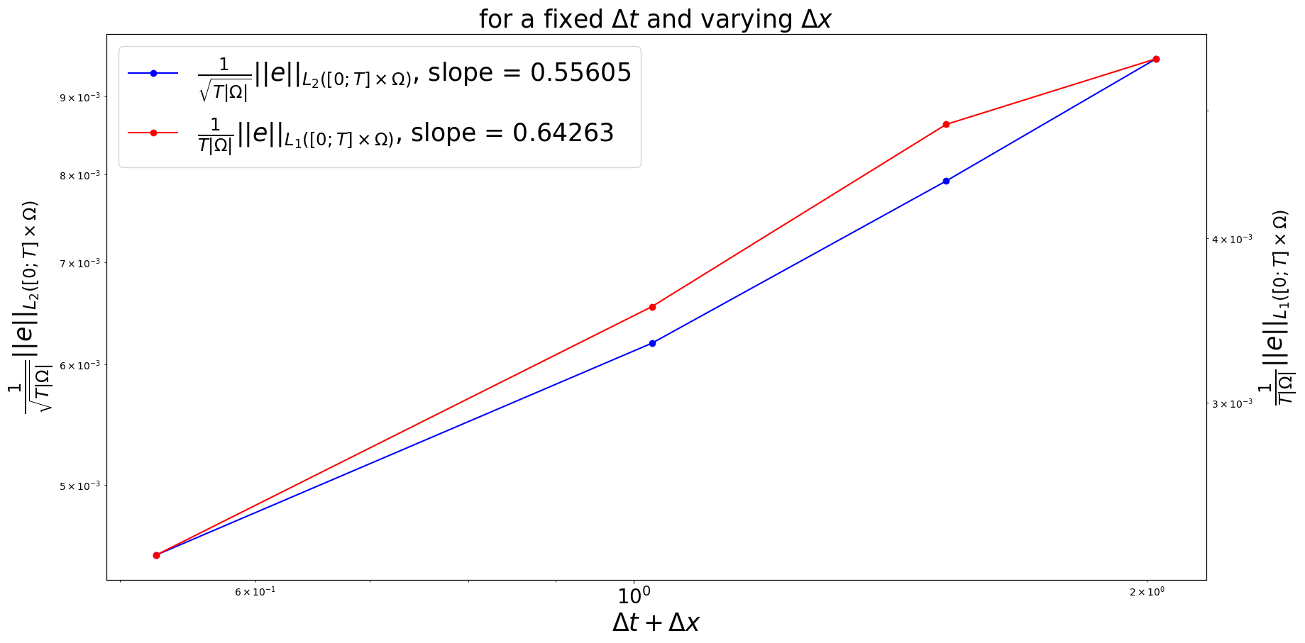
Analysis of the error estimate

In this section, the estimate of the error \(e(x,y,t)=|p^{solver}(x,y,t)-p^{ref}(x,y,t)|\) is analyzed.

Analysis of the error estimate for several space step

[9]:

coeff_dx_a = [0.5, 1., 1.5, 2.]
abs_a = np.zeros((len(coeff_dx_a)))

MAE_vs_space_step = np.zeros((len(coeff_dx_a)))
RMSE_vs_space_step = np.zeros((len(coeff_dx_a)))


for i, coeff_dx in enumerate(coeff_dx_a):

    msh = MeshRect2D(Lx, Ly, Delta_x * coeff_dx, Delta_y * coeff_dx, T_final)

    model_adjoint, cost = EDP(msh, 0.025)

    p_ref = p_reference(msh)

    abs_a[i] = msh.dx + msh.dt
    print("")
    print("dx = ", msh.dx)
    print("dt = ", msh.dt)

    p_solver = model_adjoint.solver(cost.obs.adjoint_derivative_obs_operator, cost)
    p_solver = p_solver.reshape((msh.t_array.size, msh.y.size, msh.x.size))

    RMSE_vs_space_step[i] = npl.norm(p_solver - p_ref) / np.sqrt(p_solver.size)
    MAE_vs_space_step[i] = np.mean(np.abs(p_solver - p_ref))

/home/tmalou/anaconda3/envs/pherosensor-new/lib/python3.7/site-packages/pherosensor-0.1.1-py3.7.egg/pheromone_dispersion/diffusion_tensor.py:55: RuntimeWarning: invalid value encountered in true_divide
  U_at_vertical_interface = self.U.at_vertical_interface / norm_U_at_vertical_interface[:, :, None]
/home/tmalou/anaconda3/envs/pherosensor-new/lib/python3.7/site-packages/pherosensor-0.1.1-py3.7.egg/pheromone_dispersion/diffusion_tensor.py:74: RuntimeWarning: invalid value encountered in true_divide
  U_at_horizontal_interface = self.U.at_horizontal_interface / norm_U_at_horizontal_interface[:, :, None]


dx =  0.5
dt =  0.025
t = 0.000 / 2.000 s
dx =  1.0
dt =  0.025
t = 0.000 / 2.000 s
dx =  1.5
dt =  0.025
t = 0.000 / 2.000 s
dx =  2.0
dt =  0.025
t = 0.000 / 2.000 s

[10]:

slope_MAE_vs_space_step = ( np.log(MAE_vs_space_step[0]) - np.log(MAE_vs_space_step[-1]) ) / ( np.log(abs_a[0]) - np.log(abs_a[-1]) )
slope_RMSE_vs_space_step = ( np.log(RMSE_vs_space_step[0]) - np.log(RMSE_vs_space_step[-1]) ) / ( np.log(abs_a[0]) - np.log(abs_a[-1]) )

fontsize = 25
fig, ax1 = plt.subplots(figsize=(20, 10))

ax1.plot(abs_a,RMSE_vs_space_step,'-ob',label=r'$\frac{1}{\sqrt{T|\Omega|}}||e||_{L_2([0;T]\times\Omega)}$'+f', slope = {"{:.5f}".format(slope_RMSE_vs_space_step)}')
ax1.tick_params(axis='both',labelsize=fontsize-5)
ax1.set_ylabel(r'$\frac{1}{\sqrt{T|\Omega|}}||e||_{L_2([0;T]\times\Omega)}$', fontsize=fontsize)
ax1.set_xlabel('$\Delta t + \Delta x$', fontsize=fontsize)
ax1.set_xscale('log')
ax1.set_yscale('log')
ax1.set_title(r'for a fixed $\Delta t$ and varying $\Delta x$', fontsize=fontsize)

ax2 = ax1.twinx()
ax2.plot(abs_a,MAE_vs_space_step,'-or',label=r'$\frac{1}{T|\Omega|}||e||_{L_1([0;T]\times\Omega)}$'+f', slope = {"{:.5f}".format(slope_MAE_vs_space_step)}')
ax2.tick_params(axis='both',labelsize=fontsize-5)
ax2.set_ylabel(r'$\frac{1}{T|\Omega|}||e||_{L_1([0;T]\times\Omega)}$', fontsize=fontsize)
ax2.set_yscale('log')

line1, label1 = ax1.get_legend_handles_labels()
line2, label2 = ax2.get_legend_handles_labels()
ax2.legend(line1+line2,label1+label2,loc='upper left',prop={'size': fontsize})#, bbox_to_anchor=(1.17,1.1)

[10]:

<matplotlib.legend.Legend at 0x7f4383188250>

../../_images/tutorials_test_numerical_scheme_test_EDP_model_adjoint_14_1.png

[ ]: