[1]:
import matplotlib.pyplot as plt
from matplotlib import ticker
import numpy as np
import numpy.linalg as npl
from scipy.sparse.linalg import cg

import pherosensor

from pheromone_dispersion.diffusion_operator import Diffusion
from pheromone_dispersion.diffusion_tensor import DiffusionTensor
from pheromone_dispersion.geom import MeshRect2D
from pheromone_dispersion.velocity import Velocity
[2]:
Lx = 20
Ly = 25
Delta_x = 0.4
Delta_y = 0.4
T_final = 5.
Test of the numerical scheme of the diffusion operator
This notebook aims to test the implementation of the numerical scheme of the diffusion operator.
The diffusion operator is the operator \(D:c\mapsto \nabla\cdot(\mathbf{K}(x,y)\nabla c(x,y))~\forall (x,y)\in\Omega\) such that \(K\nabla c\cdot \vec{n} = 0~\forall(x,y)\in\partial\Omega\).
Reference solution
[3]:
K_x = 5./3.
K_y = 1.

def diffusion_tensor(msh):

    U_hi = np.zeros((msh.y_horizontal_interface.size,msh.x.size,2))
    U_hi[:,:,0] = 1.
    U_vi = np.zeros((msh.y.size,msh.x_vertical_interface.size,2))
    U_vi[:,:,0] = 1.
    U = Velocity(msh, U_vi, U_hi)
    return DiffusionTensor(U, K_x, K_y)
We also consider the reference solution \(c^{ref}(x,y,t) = cos\left(\frac{2\pi n_xx}{L_x}\right)+cos\left(\frac{2\pi n_yy}{L_y}\right)\).
[4]:
nx = 5
ny = 7
lambda_x = 2 * np.pi * nx / Lx
lambda_y = 2 * np.pi * ny / Ly

def c_reference(x,y):
    return np.cos(lambda_x * x) + np.cos(lambda_y * y)
Hence, we have \(Dc^{ref}(x,y) = \nabla\cdot(\mathbf{K}\nabla c^{ref}) = -K_x\frac{4\pi^2 n_x^2}{L_x^2}cos\left(\frac{2\pi n_xx}{L_x}\right)-K_y\frac{4\pi^2 n_y^2}{L_y^2}cos\left(\frac{2\pi n_yy}{L_y}\right)\)
[5]:
def Dc_reference(x,y):
    return - K_x * lambda_x**2 * np.cos(lambda_x * x) - K_y * lambda_y**2 * np.cos(lambda_y * y)
Numerical scheme
[6]:
space_factor_a = [0.005, 0.01, 0.1, 1.]
dx_a = np.zeros(len(space_factor_a))

MAE = np.zeros(len(space_factor_a))
RMSE = np.zeros(len(space_factor_a))

for i, space_factor in enumerate(space_factor_a):

    msh = MeshRect2D(Lx, Ly, Delta_x*space_factor, Delta_y*space_factor, T_final)
    dx_a[i] = Delta_x*space_factor
    x, y = np.meshgrid(msh.x, msh.y)

    c_ref = c_reference(x,y)
    Dc_ref = Dc_reference(x,y)

    K = diffusion_tensor(msh)
    D = Diffusion(K, msh)
    Dc_solver = D.matvec(c_ref.reshape((msh.y.size * msh.x.size,)))
    Dc_solver = Dc_solver.reshape((msh.y.size, msh.x.size))

    MAE[i] = np.mean(np.abs(Dc_solver - Dc_ref))
    RMSE[i] = npl.norm(Dc_solver - Dc_ref) / np.sqrt(Dc_ref.size)

    print("")
    print("dx = ", msh.dx)
dx =  0.002

dx =  0.004

dx =  0.04000000000000001

dx =  0.4
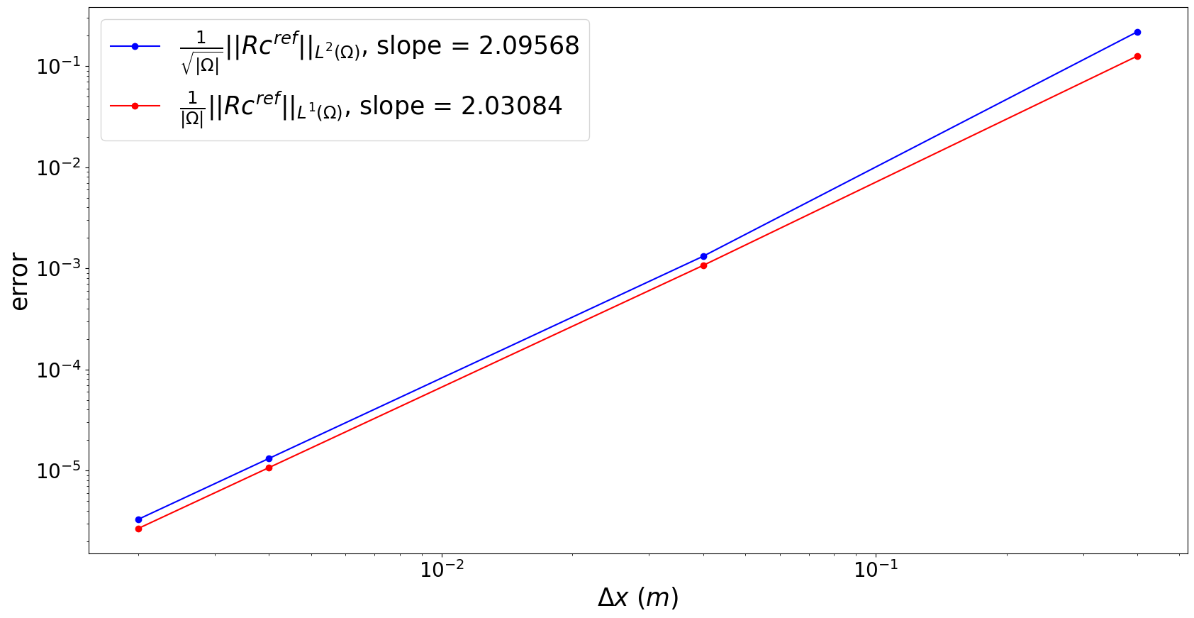
Analysis of the truncation error
[7]:
slope_MAE = (np.log(MAE[0]) - np.log(MAE[-1])) / (np.log(dx_a[0]) - np.log(dx_a[-1]))
slope_RMSE = (np.log(RMSE[0]) - np.log(RMSE[-1]) ) / ( np.log(dx_a[0]) - np.log(dx_a[-1]))

fontsize = 25
fig, ax1 = plt.subplots(figsize=(20, 10))

ax1.plot(dx_a,RMSE,'-ob',label=r'$\frac{1}{\sqrt{|\Omega|}}||Rc^{ref}||_{L^2(\Omega)}$'+f', slope = {"{:.5f}".format(slope_RMSE)}')
ax1.plot(dx_a,MAE,'-or',label=r'$\frac{1}{|\Omega|}||Rc^{ref}||_{L^1(\Omega)}$'+f', slope = {"{:.5f}".format(slope_MAE)}')
ax1.tick_params(axis='both',labelsize=fontsize-5)
ax1.set_ylabel(r'error', fontsize=fontsize)
ax1.set_xlabel('$\Delta x$ ($m$)', fontsize=fontsize)
ax1.set_xscale('log')
ax1.set_yscale('log')
ax1.legend(loc='upper left',prop={'size': fontsize})
[7]:
<matplotlib.legend.Legend at 0x758460554a90>
Scalar product test for the adjoint of the diffusion operator
Let us note that the diffusion operator is auto-adjoint: \(D^*=D\), for a symmetric diffusion tensor \(\mathbf{K}=\mathbf{K}^T\).
This section aims at performing the scalar product test for the diffusion operator. It also enables to check that the scheme of the diffusion operator is also auto-adjoint.
The test of the scalar product consists in checking that \(<Dc_1,c_2>\approx<c_1,D^*c_2>\) for any \(c_1\) and \(c_2\) (here picked randomly).
[8]:
msh = MeshRect2D(Lx, Ly, Delta_x, Delta_y, T_final)
K = diffusion_tensor(msh)

D = Diffusion(K, msh)

np.random.seed(0)
c1 = np.random.normal(0, 1, size=msh.x.size*msh.y.size)
c2 = np.random.normal(0, 1, size=msh.x.size*msh.y.size)

prod_scal_D = np.dot(c2,D.matvec(c1))
prod_scal_DT = np.dot(c1,D.matvec(c2))

print("<Dc_1,c_2> = ",prod_scal_D)
print("<c_1,D*c_2> = ",prod_scal_DT)
print("|<Dc_1,c_2>-<c_1,D*c_2>| = ", np.abs(prod_scal_D-prod_scal_DT))
<Dc_1,c_2> =  1902.906719677645
<c_1,D*c_2> =  1902.9067196776446
|<Dc_1,c_2>-<c_1,D*c_2>| =  4.547473508864641e-13